39 excel chart change all data labels at once

chandoo.org › wp › change-data-labels-in-chartsHow to Change Excel Chart Data Labels to Custom Values? Now, click on any data label. This will select "all" data labels. Now click once again. At this point excel will select only one data label. Go to Formula bar, press = and point to the cell where the data label for that chart data point is defined. Repeat the process for all other data labels, one after another. See the screencast. Points to note: how to add data labels into Excel graphs — storytelling with data To adjust the number formatting, navigate back to the Format Data Label menu and scroll to the Number section at the bottom. I'll choose Number in the Category drop-down and change Decimal places to 0 (side note: checking the Linked to source box is a good option if you want the labels to reformat when the formatting of the underlying source data changes).

Formating all data labels in a single series at once. Easiest way to make sure you are doing the right thing is to click off the data labels but on the chart and then right click any data label and choose Format Data Labels. Note the choice on the shortcut menu should not say Format Data Label. What's the difference? the "s" at the end.

Excel chart change all data labels at once

change format for all data series in chart [SOLVED] It might depend on the kind of format change you are trying to do. The only "chart wide" command I can think of is the "change chart type" command. So, if you have a scatter chart with markers and no lines and you want to add lines to each data series, you could go into the change chart type, and change to a scatter with markers and lines. Change the position of data labels automatically Click the chart outside of the data labels that you want to change. Click one of the data labels in the series that you want to change. On the Format menu, click Selected Data Labels, and then click the Alignment tab. In the Label position box, click the location you want. previous page start next page. peltiertech.com › multiple-time-series-excel-chartMultiple Time Series in an Excel Chart - Peltier Tech Aug 12, 2016 · This discussion mostly concerns Excel Line Charts with Date Axis formatting. Date Axis formatting is available for the X axis (the independent variable axis) in Excel’s Line, Area, Column, and Bar charts; for all of these charts except the Bar chart, the X axis is the horizontal axis, but in Bar charts the X axis is the vertical axis.

Excel chart change all data labels at once. Custom Data Labels with Colors and Symbols in Excel Charts - [How To ... Step 4: Select the data in column C and hit Ctrl+1 to invoke format cell dialogue box. From left click custom and have your cursor in the type field and follow these steps: Press and Hold ALT key on the keyboard and on the Numpad hit 3 and 0 keys. Let go the ALT key and you will see that upward arrow is inserted. Excel changes multiple series colors at once sub formatseriesthesame() if activechart is nothing then msgbox "select a chart and try again!", vbexclamation goto exitsub end if with activechart dim icolor as long icolor = .seriescollection(2).format.line.forecolor.rgb dim iseries as long for iseries = 3 to .seriescollection.count .seriescollection(iseries).format.line.forecolor.rgb = icolor … Excel chart changing all data labels from value to series name ... By selecting chart then from layout->data labels->more data labels options ->label options ->label contains-> (select)series name, I can only get one series name replacing its respective label values. For more than hundred series stacked in columns i want them all to be changed at once, is there any way out? why it does not change them all at once? Change the labels in an Excel data series | TechRepublic Click the Chart Wizard button in the Standard toolbar. Click Next. Click the Series tab. Click the Window Shade button in the Category (X) Axis. Labels box. Select B3:D3 to select the labels in ...

Excel 2010: How to format ALL data point labels SIMULTANEOUSLY Instead of selecting the entire chart, right click one of the data points and select "Format Data Labels". B brianclong Board Regular Joined Apr 11, 2006 Messages 168 May 24, 2011 #3 This still only formats one set of data series labels. Maybe there's a bug? I have Office 64 bit. G gehusi Board Regular Joined Jul 20, 2010 Messages 182 May 24, 2011 support.microsoft.com › en-us › officeEdit titles or data labels in a chart - support.microsoft.com You can also place data labels in a standard position relative to their data markers. Depending on the chart type, you can choose from a variety of positioning options. On a chart, do one of the following: To reposition all data labels for an entire data series, click a data label once to select the data series. How to Customize Your Excel Pivot Chart Data Labels - dummies The Data Labels command on the Design tab's Add Chart Element menu in Excel allows you to label data markers with values from your pivot table. When you click the command button, Excel displays a menu with commands corresponding to locations for the data labels: None, Center, Left, Right, Above, and Below. None signifies that no data labels ... How to add or move data labels in Excel chart? - ExtendOffice In Excel 2013 or 2016. 1. Click the chart to show the Chart Elements button . 2. Then click the Chart Elements, and check Data Labels, then you can click the arrow to choose an option about the data labels in the sub menu. See screenshot: In Excel 2010 or 2007. 1. click on the chart to show the Layout tab in the Chart Tools group. See ...

How to set multiple series labels at once - Microsoft Tech Community Click anywhere in the chart. On the Chart Design tab of the ribbon, in the Data group, click Select Data. Click in the 'Chart data range' box. Select the range containing both the series names and the series values. Click OK. If this doesn't work, press Ctrl+Z to undo the change. 0 Likes Reply Nathan1123130 replied to Hans Vogelaar Format Data Labels in Excel- Instructions - TeachUcomp, Inc. To format data labels in Excel, choose the set of data labels to format. To do this, click the "Format" tab within the "Chart Tools" contextual tab in the Ribbon. Then select the data labels to format from the "Chart Elements" drop-down in the "Current Selection" button group. Then click the "Format Selection" button that ... excel - Change format of all data labels of a single series at once ... Go straight back to the same data series and right mouse click, and choose add data labels This has worked in Excel 2016. Purely by luck I worked this out saving a great deal of time and frustration. Share answered May 9, 2018 at 13:51 Nic 185 1 9 Add a comment Excel charts: add title, customize chart axis, legend and data labels For example, this is how we can add labels to one of the data series in our Excel chart: For specific chart types, such as pie chart, you can also choose the labels location. For this, click the arrow next to Data Labels, and choose the option you want. To show data labels inside text bubbles, click Data Callout. How to change data displayed on ...

Mapping relationships between people using interactive network chart » Chandoo.org - Learn Excel ...

change all data labels - Excel Help Forum For a new thread (1st post), scroll to Manage Attachments, otherwise scroll down to GO ADVANCED, click, and then scroll down to MANAGE ATTACHMENTS and click again. Now follow the instructions at the top of that screen. New Notice for experts and gurus:

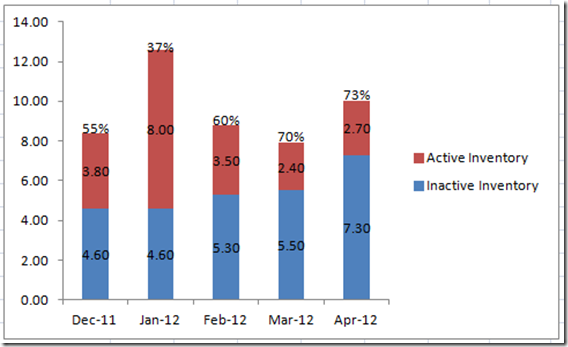
How-to Put Percentage Labels on Top of a Stacked Column Chart - Excel Dashboard Templates

› documents › excelHow to change chart axis labels' font color and size in Excel? We can easily change all labels' font color and font size in X axis or Y axis in a chart. Just click to select the axis you will change all labels' font color and size in the chart, and then type a font size into the Font Size box, click the Font color button and specify a font color from the drop down list in the Font group on the Home tab ...

Art of Charts: Building bubble grid charts in Excel 2016

How to add data labels from different column in an Excel chart? Click any data label to select all data labels, and then click the specified data label to select it only in the chart. 3. Go to the formula bar, type =, select the corresponding cell in the different column, and press the Enter key. See screenshot: 4. Repeat the above 2 - 3 steps to add data labels from the different column for other data points.

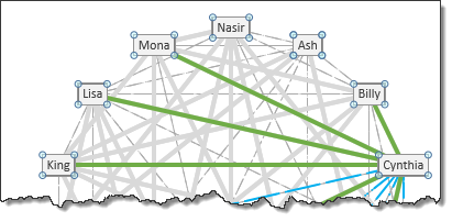
Mapping relationships between people using interactive network chart | Chandoo.org - Learn ...

› dynamically-labelDynamically Label Excel Chart Series Lines • My Online ... Sep 26, 2017 · To modify the axis so the Year and Month labels are nested; right-click the chart > Select Data > Edit the Horizontal (category) Axis Labels > change the ‘Axis label range’ to include column A. Step 2: Clever Formula. The Label Series Data contains a formula that only returns the value for the last row of data.

Share :