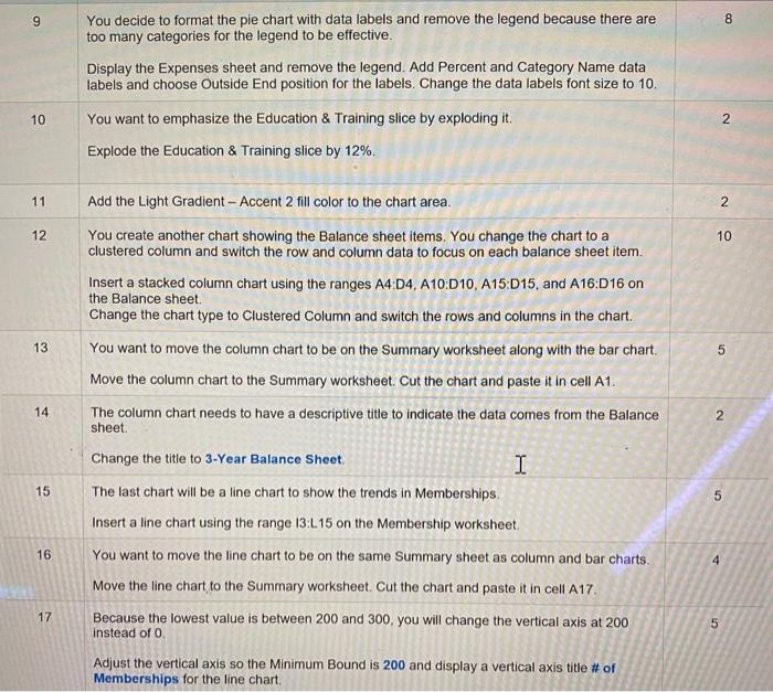
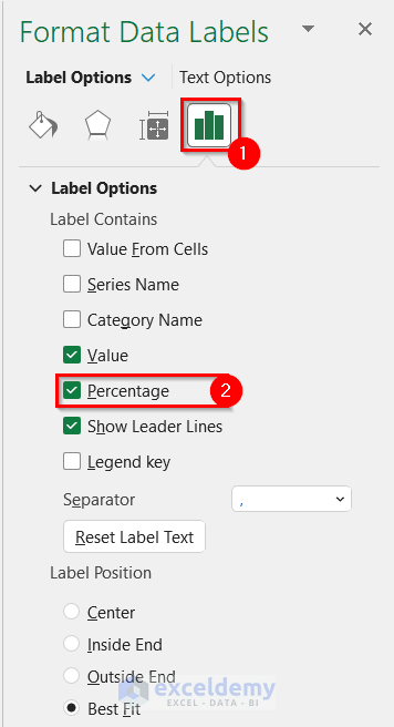
38 use the format data labels task pane to display category name and percentage data labels
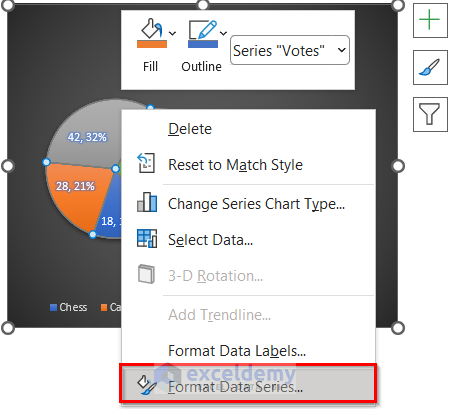
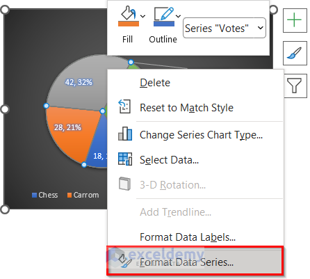
PDF Where is the format data labels task pane in excel "Green" means 0 will turn to green, and you can change all color names based on your needs. 3. Close the Format Axis pane or Format Axis dialog box. Then all labels' font color are changed based on the format code in the selected axis. See below screen shot: Change axis labels' font color if greater or less than value with conditional ... (Get Answer) - Share Format Data Labels Display Outside End data labels ... Share Format Data Labels Display Outside End data labels on the pie chart. Close the Chart Elements menu. Use the Format Data Labels task pane to display Percentage data labels and remove the Value data labels. Close the task pane.
Formal ALL data labels in a pivot chart at once I go through the post, as per the article: Change the format of data labels in a chart, you may select only one data labels to format it. However, you may change the location of the data labels all at once, as you can see in screenshot below: I would suggest you vote for or leave your comments in the thread: Format Data Labels (Ex: Alignment ...
Use the format data labels task pane to display category name and percentage data labels
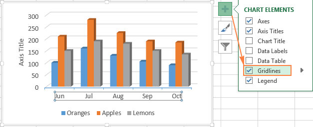
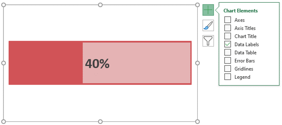
How to show percentages on three different charts in Excel In the Chart Elements menu, hover your cursor over the Data Labels option and click on the arrow next to it. 4. In the opened submenu, click on More options. This opens the Format Data Labels task pane. 5. In the Format Data Labels task pane, untick Value and tick the Percentage option to show only percentages. What Is The Format Task Pane In Excel? | Knologist The second thing you need to do is to select the data you want to format. Then, you can click on the conditional formatting tool. This will select the data you've selected in the first step. The third thing you need to do is to click on the Format Cells button. This button will change the data in the cells in the table to the color you've selected. cs 385 exam 3 Flashcards | Quizlet data tab, subtotal, click at each change in: select area, unselect replace current subtotals, click ok Collapse the table to show the grand totals only. click 1 at top left corner Expand the table to show the grand and discipline totals. click 2 at top left corner Use the Auto Outline feature to group the columns.
Use the format data labels task pane to display category name and percentage data labels. Excel tutorial: The Format Task pane You can also select a chart element first, then use the keyboard shortcut Control + 1. For example, if I select the data bars in this chart, then type Control + 1, the Format Task Pane will open with with the data series options selected. The Format Task pane stays open until you manually close the window. Format Data Label Options in PowerPoint 2013 for Windows - Indezine Alternatively, select data labels of any data series in your chart and right-click to bring up a contextual menu, as shown in Figure 2, below. From this menu, choose the Format Data Labels option. Either of these options opens the Format Data Labels Task Pane, as shown in Figure 3, below. Formatting Data Labels Right-Click Menu: Right-click a series on the chart, point to Data Labels, and then select Show . To hide data labels, right-click a series on the chart, point to Data Labels, and then select Hide. The data labels appear, and are formatted and styled accordingly. The following image shows a chart with data labels. Display the percentage data labels on the active chart. - YouTube Display the percentage data labels on the active chart.Want more? Then download our TEST4U demo from TEST4U provides an innovat...
A data label is descriptive text that shows that - Course Hero To format the data labels - Double click a data label to open the Format Data Labels task pane. Click the Label Options Icon. Click Label Options to customize the labels, and complete any of the following steps: Select the Label Contains options. The default is Value, but you might want to display additional label contents, such as Category Name. How to: Display and Format Data Labels - DevExpress In particular, set the DataLabelBase.ShowCategoryName and DataLabelBase.ShowPercent properties to true to display the category name and percentage value in a data label at the same time. To separate these items, assign a new line character to the DataLabelBase.Separator property, so the percentage value will be automatically wrapped to a new line. Solved option to change the In the Format Data Labels task - Chegg Expert Answer. Solution: Effects and 3-D Format …. View the full answer. Transcribed image text: option to change the In the Format Data Labels task pane, use the appearance of a data label's 3-D format. Format data labels task pane Jobs, Employment | Freelancer Search for jobs related to Format data labels task pane or hire on the world's largest freelancing marketplace with 20m+ jobs. It's free to sign up and bid on jobs.
How to show data label in "percentage" instead of - Microsoft Community Select Format Data Labels Select Number in the left column Select Percentage in the popup options In the Format code field set the number of decimal places required and click Add. (Or if the table data in in percentage format then you can select Link to source.) Click OK Regards, OssieMac Report abuse 8 people found this reply helpful · Add or remove data labels in a chart - support.microsoft.com Right-click the data series or data label to display more data for, and then click Format Data Labels. Click Label Options and under Label Contains, select the Values From Cells checkbox. When the Data Label Range dialog box appears, go back to the spreadsheet and select the range for which you want the cell values to display as data labels. excel 2,3 Flashcards | Quizlet You must make changes to the content of data labels using buttons in the Format Data Labels task pane. true Excel offers two pie chart sub-types, Pie of Pie and Bar of Bar, that can be used to combine many smaller segments of a pie chart into a separate smaller chart. false How do I change axis labels to months? - Firstlawcomic Using either method then displays the "Format Data Labels" task pane at the right side of the screen. How do you display the data labels on this chart above the data markers? Click the chart, and then click the Chart Design tab. Click Add Chart Element and select Data Labels, and then select a location for the data label option.
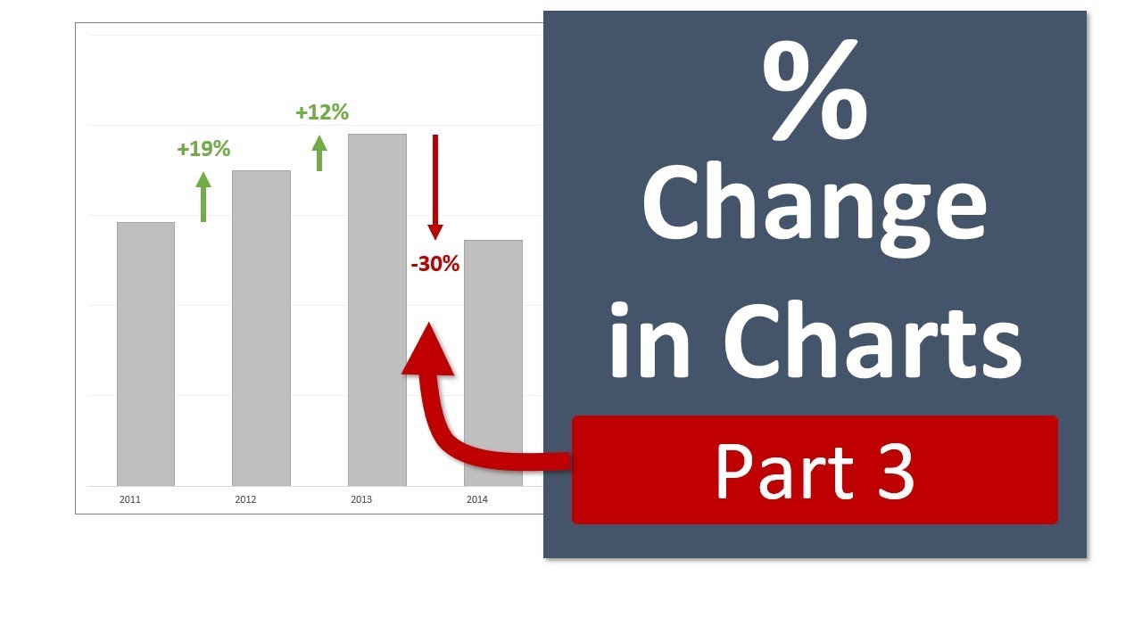
Column Chart That Displays Percentage Change or Variance ...
How to use data labels - Exceljet When first enabled, data labels will show only values, but the Label Options area in the format task pane offers many other settings. You can set data labels to show the category name, the series name, and even values from cells. In this case for example, I can display comments from column E using the "value from cells" option.

How to create a chart with both percentage and value in Excel?
How do I display the format data Labels Task Pane? - Heimduo How do I add data labels in Excel? 1. Right click the data series in the chart, and select Add Data Labels > Add Data Labels from the context menu to add data labels. 2. Click any data label to select all data labels, and then click the specified data label to select it only in the chart. How do you put data labels on top of bars in Powerpoint?

How to make a pie chart in Excel
Format Data Labels in Excel- Instructions - TeachUcomp, Inc. To format data labels in Excel, choose the set of data labels to format. To do this, click the "Format" tab within the "Chart Tools" contextual tab in the Ribbon. Then select the data labels to format from the "Chart Elements" drop-down in the "Current Selection" button group.
Microsoft Excel Charting
PDF Use the format data labels task pane to display category name 3. Right-click in the chart area, then select Add Data Labels and click Add Data Labels in the popup menu: 4. Click in one of the labels to select all of them, then right-click and select Format Data Labels... in the popup menu: 5. On the Format Data Labels pane, in the Label Options tab, select the Category Name checkbox: 6.

Creating Pie Chart and Adding/Formatting Data Labels (Excel)
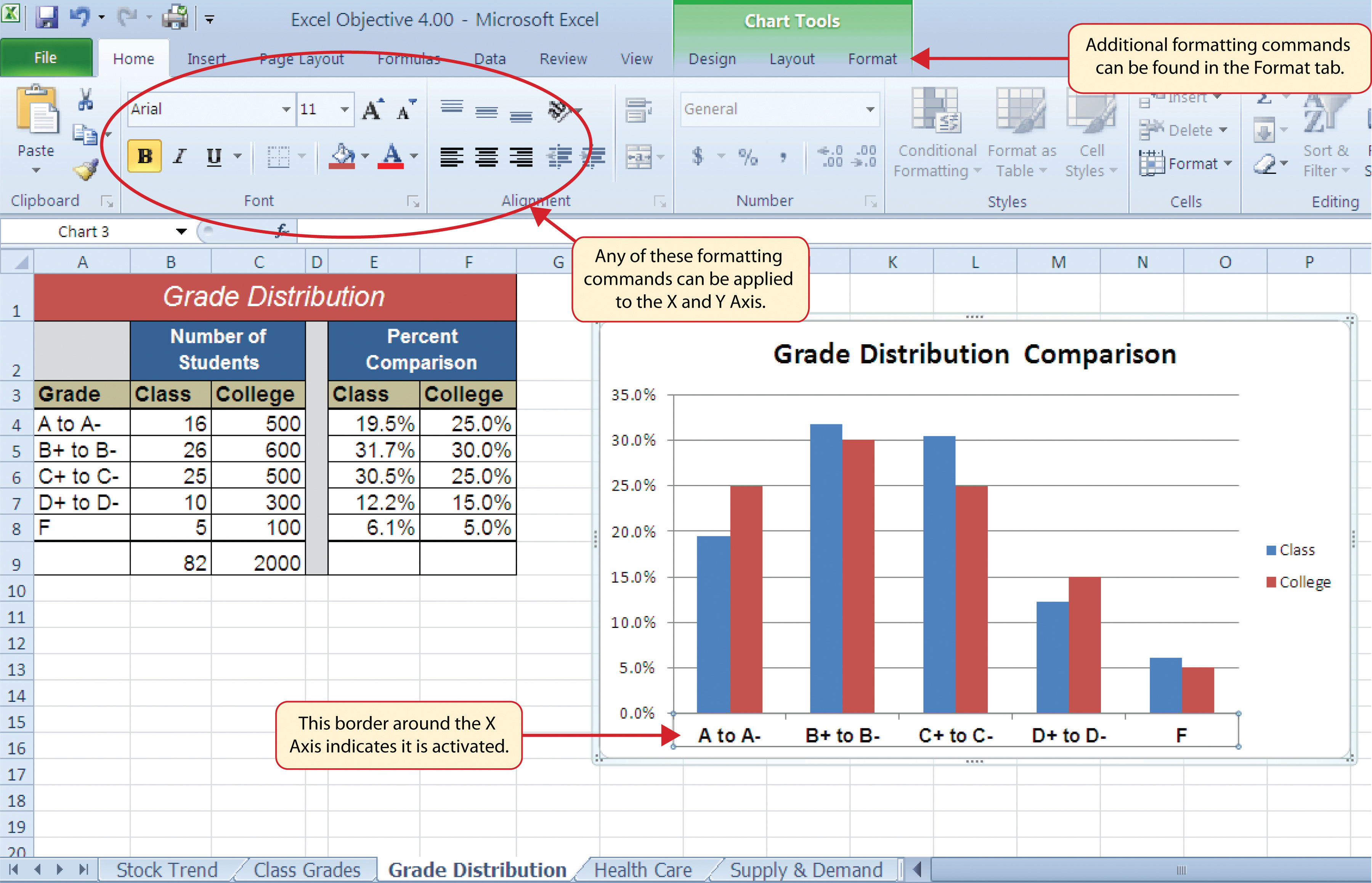
Solved step by step instruction 2 A pie chart is an | Chegg.com Use the Insert tab to create a pie chart from the Question: step by step instruction 2 A pie chart is an effective way to visually illustrate the percentage of the class that earned A, B, C, D, and F grades. Use the Insert tab to create a pie chart from the This problem has been solved! See the answer step by step instruction Expert Answer

Display Customized Data Labels on Charts & Graphs
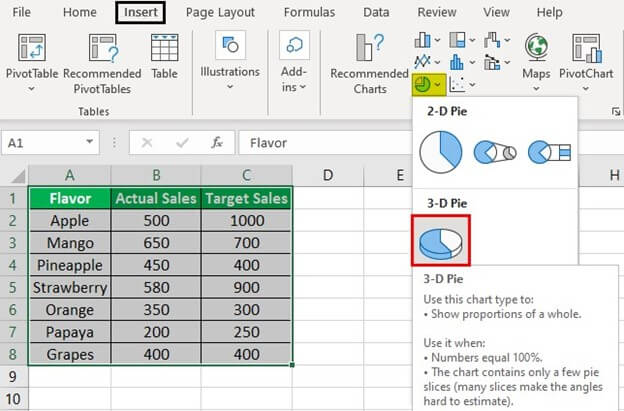
Excel 3-D Pie charts - Microsoft Excel 2016 - OfficeToolTips 2. On the Insert tab, in the Charts group, choose the Pie button: Choose 3-D Pie. 3. Right-click in the chart area, then select Add Data Labels and click Add Data Labels in the popup menu: 4. Click in one of the labels to select all of them, then right-click and select Format Data Labels... in the popup menu: 5.

How to Create Multi-Category Chart in Excel - Excel Board
How to use Aesthetic Data Labels - JT Scientific To format a single data label −. Step 1 − Click twice any data label you want to format. Step 2 − Right-click that data label and then click Format Data Label. Alternatively, you can also click More Options in data labels options to display on the Format Data Label task pane. There are many formatting options for data labels in the format ...

Apply Custom Data Labels to Charted Points - Peltier Tech
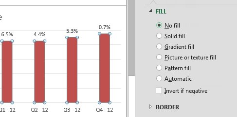
Change the format of data labels in a chart To get there, after adding your data labels, select the data label to format, and then click Chart Elements > Data Labels > More Options. To go to the appropriate area, click one of the four icons ( Fill & Line, Effects, Size & Properties ( Layout & Properties in Outlook or Word), or Label Options) shown here.
Step Instructions Points Possible 1 1 0 Start Excel. | Chegg.com
UsetheFormatDataLabelstaskpanetodisplay | Course Hero Use the Format Data Labels task pane to display Percentage data labels and remove the Value data labels. Close the task pane. Apply 18 point size to the data labels. a. Click green plus data labels center click green plus double click in chart label contains click percentage click values check box click close click home font 18 9.

How to create a chart with both percentage and value in Excel?
cs 385 exam 3 Flashcards | Quizlet data tab, subtotal, click at each change in: select area, unselect replace current subtotals, click ok Collapse the table to show the grand totals only. click 1 at top left corner Expand the table to show the grand and discipline totals. click 2 at top left corner Use the Auto Outline feature to group the columns.

Apply Custom Data Labels to Charted Points - Peltier Tech
What Is The Format Task Pane In Excel? | Knologist The second thing you need to do is to select the data you want to format. Then, you can click on the conditional formatting tool. This will select the data you've selected in the first step. The third thing you need to do is to click on the Format Cells button. This button will change the data in the cells in the table to the color you've selected.

How to make a pie chart in Excel
How to show percentages on three different charts in Excel In the Chart Elements menu, hover your cursor over the Data Labels option and click on the arrow next to it. 4. In the opened submenu, click on More options. This opens the Format Data Labels task pane. 5. In the Format Data Labels task pane, untick Value and tick the Percentage option to show only percentages.
Presenting Data with Charts

Change the format of data labels in a chart

How to show percentages on three different charts in Excel ...

How to Use Cell Values for Excel Chart Labels

Excel charts: add title, customize chart axis, legend and ...
Is it possible to adjust the data label text box dimension in ...
How to get an Excel chart to display percentages of each ...
Pie Charts in Excel - How to Make with Step by Step Examples

Change the format of data labels in a chart

Excel charts: add title, customize chart axis, legend and ...

How to create a chart with both percentage and value in Excel?

Adding rich data labels to charts in Excel 2013 | Microsoft ...
How to Make a Pie Chart in Excel (5 Suitable Examples)
Excel charts: add title, customize chart axis, legend and ...
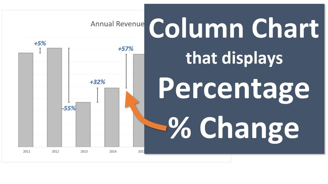
Column Chart That Displays Percentage Change or Variance ...
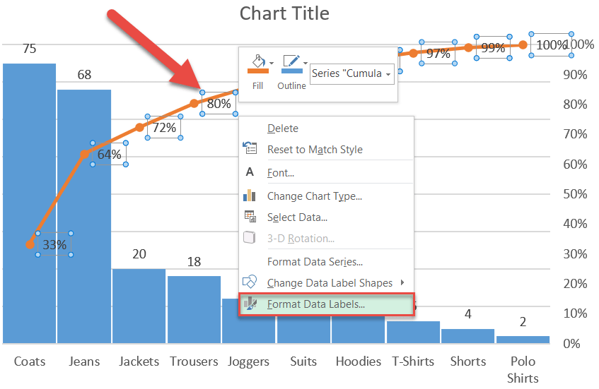
How to Create a Pareto Chart in Excel – Automate Excel
How to Make a Pie Chart in Excel (5 Suitable Examples)

Change the format of data labels in a chart

How to show percentages on three different charts in Excel ...

Change the format of data labels in a chart
How to Make a Pie Chart in Excel (5 Suitable Examples)

How to Add Data Labels to an Excel 2010 Chart - dummies

Format Data Labels in Excel- Instructions - TeachUcomp, Inc.
How To Create Excel Progress Bar Charts (Professional-Looking!)

Formatting Data Labels
Adding Extra Layers of Analysis to Your Excel Charts - dummies
Post a Comment for "38 use the format data labels task pane to display category name and percentage data labels"